The Plot 1 Window
Clicking on "Plot 1 Window" in the main window, opens up the Plot 1 Window, where numerical solutions can be plotted in the Plotting Window.
The system of ODEs from the "Main Window" is copied and used here. After opening the Plot 1 Window, any changes made on the Main Window are not updated on the Plot 1 Window. (This is different from what happens in the Numerics Window).
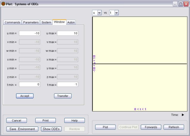
The Plot 1 Window
Above the Plotting Window you can select the variables that you want to use on the vertical and horizontal axes. The ODE that is being used here is
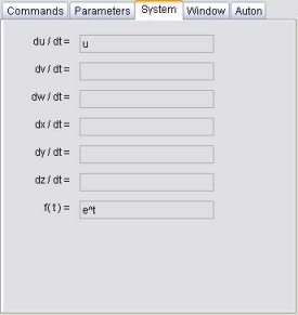
du/dt = u, u(t0) = 1, t0 = 0, t1 = 1,
with s = 0.01 and f(t) = et, so "u" and "t" are selected automatically.
Below the Plotting Window, and to the right, is "Time" followed by an arrow, in this case pointing to the right. This means that plotting will be "forwards" in time. If the arrow points to the left, then plotting will be "backwards" in time.
To the left of the Plotting Window are various tabs. The one that is exposed is the "Window" tab, which is where the minimum and maximum of each variable's window can be set. The default is -10 to 10 for each variable except "t", which defaults to "t0" and "t1". Note that the minimum and maximum of "t" need not coincide with "t0" and "t1".
The other tabs are
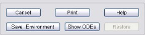
There are 6 buttons at the bottom left of the Plotting Window.
- "Cancel", which closes the Plot 1 Window.
- "Print", which allows you to print the Plot 1 Window to a printer (as long as the window has not been resized), or to a file. Various graphics file types are available: BMP, GIF, JPEG, PNG, TIFF, and WMF.
- "Help", which shows this help file.
- "Save Environment", which saves the existing ODEs (and the graphical environment) to disk with extension "en1". (The environment includes such things as the variables selected for the axes, the maximum and minimum for these variables, and the selected tab.) These are the files that can be loaded later using "Open Environment" under the "Main Window".
- "Show ODEs", which shows the current ODEs, initial values, parameters in use, etc.
- "Restore", which restores the Plot 1 Window to its original size so that printing to a printer can be enabled.
There are 4 buttons at the bottom right of the Plotting Window. These buttons are duplicated in the "Commands" tab.
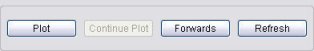
- "Plot", which plots the numerical solution to the ODE in the chosen Plotting Window, based on the selection made in "Methods" under the "Commands" Tab. The color of the plot depends on the method selected: Euler in red, Heun in green, and RK4 in blue.
- "Continue Plot", which becomes available after a plot. It continues plotting the numerical solution using the final values of the variables from the previous plot become the new initial variables of the current plot. It is equivalent to "t1 to t0" on the Numerics Window.
- "Forwards", which means that plotting will be "forwards" in time, as is indicated by arrow alongside "Time" at the bottom of the Plotting Window. Clicking the "Forwards" button changes the direction of the arrow and the word "Forwards" is then replaced by "Backwards". If the horizontal variable is "t" and the maximum and minimum of t coincide with t0 and t1, the Plotting Window is cleared and reset to the new values. Otherwise the Plotting Window is unchanged. Pressing "Plot" then draws the ODEs in the new direction.
- "Refresh", which clears the current Plotting Window.
Calculations cease if the point is well outside the Plotting Window.
When the window is resized, the Plotting Window is cleared.
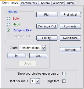
Selecting this tab shows many of the commands available for plotting ODEs.
Under "Method" there are four different numerical routines to choose from: Euler's Method, Heun's Method (sometimes called the Modified Euler's Method), Runge Kutta 4, or Adaptive RK4 (adaptive stepsize Runge Kutta 4). (Adaptive RK4 is under construction so is grayed out.)
The buttons available are:
- "Plot", which plots the numerical solution to the ODE in the chosen Plotting Window, based on the selection made in "Methods". The color of the plot depends on the method selected: Euler in red, Heun in green, and RK4 in blue. This button duplicates the "Plot" button beneath the Plotting Window.
- "Plot Initial", which places a dot at the initial point, if it is on the screen.
- "Continue Plot", which becomes available after a plot. It continues plotting the numerical solution using the final values of the variables from the previous plot become the new initial variables of the current plot. It is equivalent to "t1 to t0" on the Numerics Window. This button duplicates the "Continue Plot" button beneath the Plotting Window.
- "Forwards", which means that plotting will be "forwards" in time, as is indicated by arrow alongside "Time" at the bottom of the Plotting Window. Clicking the "Forwards" button changes the direction of the arrow and the word "Forwards" is then replaced by "Backwards". If the horizontal variable is "t" and the maximum and minimum of t coincide with t0 and t1, the Plotting Window is cleared and reset to the new values. Otherwise the Plotting Window is unchanged. Pressing Plot then draws the ODEs in the new direction. This button duplicates the "Forwards" button beneath the Plotting Window.
- "Plot f(t)", which uses the current stepsize to plot f(t) in magenta on the Plotting Window, if a function is defined and if the horizontal variable is "t".
- "Reinitialize", which restores all the values and window sizes to the initial values.
- "Refresh", which clears the current Plotting Window. This button duplicates the "Refresh" button beneath the Plotting Window.
It is possible to Zoom "In" or Zoom "Out", either "Horizontally", "Vertically", or in "Both Directions". Zooming can be undone, which also refreshes (clears) the Plotting Window.
Checking the "Show Coordinates" box, shows the coordinates as a tooltip under the mouse pointer when the mouse is over the Plotting Window. The number of decimal points displayed can be set from 1 to 10.
The coordinates under the mouse pointer when the mouse is over the Plotting Window are always displayed in the upper right. The "large Font" box, if checked, shows these coordinates in a larger bold font. The effect is immediate. This option is useful when projecting the screen in a classroom.
Clicking in the Plotting Window when the coordinates are displayed as a tooltip causes that point to become the new center of the Plotting Window, called Translating. Translating can be undone using "Undo", which also refreshes (clears) the Plotting Window.
To zoom in or out about a point other than the center of the Plotting Window, click on the point to make it the center of the screen, and then click "In" or "Out".
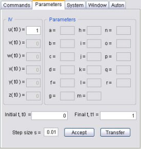
Selecting this tab shows the initial values of the dependent variables, the parameter values, the initial and final times, and the step size.
Any of these can be changed, after which the "Accept" button should be clicked.
Clicking on "Transfer", copies the values of "t0" and "t1" to "t min" and "t max" under the "Window" Tab.
Selecting this tab shows the current system of ODEs.
These values cannot be edited. To edit any of these values, close the "Plot 1 Window" and use "Edit" on the "Main Window".
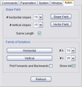
If the system of ODEs is either autonomous (the right-hand side is independent of "t") or if there is only one ODE, then this tab is exposed. Selecting this tab shows more commands grouped under Slope Field and Family of Solutions.
Slope Field.
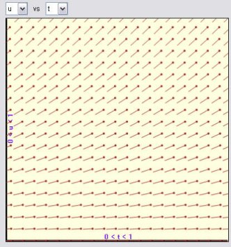
If there is only one ODE, or, in the case of an autonomous system, if "t" is not one of the variables selected in the Plotting Window, then the program will expose the "Slope Field" and "Vector Field" buttons. The number of horizontal and vertical slopes range from 5 to 40. The slopes can be of the same or variable length.
"Slope Field" plots a slope field, while "Vector Field" plots a vector field (also called a direction field). In this case, the slopes have circular heads to indicate the direction of the vector, rather like a tadpole. Here is an example
corresponding to
du/dt = u, u(t0) = 1, t0 = 0, t1 = 1.
Family of Solutions.
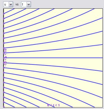
It is possible to plot a family of solutions (that is, multiple solutions) based on the current initial values and the variables selected for the horizontal and vertical axes. One of the two variables is kept fixed, while the other's maximum and minimum are divided into an equal number of new initial points. The plot uses the Method selected under the Commands Tab.
If the "Show init" box is checked, the initial points are shown.
If the "Plot Forwards and Backwards" box is checked, the solutions are plotted both forwards and backwards in time.
While plotting a family of solutions a progress bar and an "Abort" button are exposed, allowing you to stop the calculations at any time.
The original initial values are restored after the plots. Here is an example where "Vertical" is selected, and the number of vertical solutions ("# v") is 20.
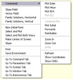
Context Menu
When the mouse is over the Plotting Window, right-clicking reveals the Context menu, which puts many of the commands available under the tabs, in one place.
The Commands to the right, are the same ones that appear under the Commands Tab.
The first group on the left-hand side are the same ones that appear under the Auton Tab.
The second group on the left-hand side depend on the position of the mouse pointer when you right-clicked to get the Context Menu.
- "New Initial Point" makes the coordinates under the pointer the new initial point, and plots this point. This menu item is visible if there is only one ODE, or, in the case of an autonomous system, if "t" is not one of the variables selected in the Plotting Window.
- "Select and Plot" makes the coordinates under the pointer the new initial point and then plots both this point and the numerical solution, based on the "Method" selected under the Commands Tab. After plotting to a window in which "t" is not one of the plot variables, the initial times are restored. This menu item is visible if there is only one ODE, or, in the case of an autonomous system, if "t" is not one of the variables selected in the Plotting Window.
- "Select and Plot Both Ways" makes the coordinates under the pointer the new initial point and then plots both this point and the numerical solution forwards and backwards, based on the "Method" selected under the Commands Tab. After plotting to a window in which "t" is not one of the plot variables, the initial times are restored. This menu item is visible if there is only one ODE, or, in the case of an autonomous system, if "t" is not one of the variables selected in the Plotting Window.
- "Make Center of Screen" makes the point under the cursor the new center of the Plotting Window. It is the same as clicking on the Plotting Window if "Show Coordinates" is checked under the Commands Tab. However, here the "Show Coordinates" need not be checked for this to work. "Undo" under the Commands Tab undoes this operation, and clears the screen.
- "Slope" draws a single slope at the pointer. This menu item is visible if there is only one ODE, or, in the case of an autonomous system, if "t" is not one of the variables selected in the Plotting Window.
The menu items in third group are the same as those displayed at the bottom left of the Plot 1 Window.
The final group allows you to rapidly move to one of the tabs.