Elliptical Instability

The behavior of rotating fluid is a ubiquitous phenomenon, arising in laboratory settings, and in geophysical and astrophysical applications. The Taylor-Proudman theorem suggests that steady, rotating flows tend to be planar. An interesting question is how does the planar flow become three dimensional? A common mechanism for the bifurcation from a planar to a fully three dimensional flow is the elliptical instability [Ker02]. Elliptical instability refers to the instability mechanism by which three dimensional flows are generated from planar flows with elliptical streamlines. The linear problem has been studied extensively in earlier work [Bay86,Ioo95,IMD90]. Our goal is to understand the possible types of nonlinear behavior that result near the bifurcation points.

We consider a rotating, inviscid, incompressible fluid in a triaxial ellipsoid ${\frac{{x_1^2}}{{a_1^2}}}$ + ${\frac{{x_2^2}}{{a_2^2}}}$ + ${\frac{{x_3^2}}{{a_3^2}}}$ $\leq$ 1. This system satisfies the Euler equation

$${\frac{{\partial \mathbf {v}}}{{\partial t}}} \nabla \nabla \nabla$$ (4)

with boundary condition v ^. n = 0. v is the velocity of the fluid, and the pressure p enforces incompressibility $\nabla$ ^. v = 0. This equation admits a planar steady state solution with elliptical streamlines:

$$\left(\vphantom{ x_2\frac{a_1}{a_2}, - x_1 \frac{a_2}{a_1},0 }\right. {\frac{{a_1}}{{a_2}}} {\frac{{a_2}}{{a_1}}} \left.\vphantom{ x_2\frac{a_1}{a_2}, - x_1 \frac{a_2}{a_1},0 }\right)$$ (5)

We will henceforth refer to this as the base flow.

There are two dimensionless parameters in this problem,

$$\mu$$ = $$\sqrt{{\frac{2 a_3^2}{a_1^2 + a_2^2}}}$$,    $$\epsilon$$ = $${\frac{{a_1^2 - a_2^2}}{{a_1^2 + a_2^2}}}$$.

The stability of this base flow depends on these parameters. The solution for the axisymmetric case ( $\epsilon$ = 0) is rigid body rotation and is stable. When $\epsilon$ $\not=$0, the flow is unstable for certain values of $\mu$. Our goal is to study the stability of the base flow, in terms of these two parameters $\mu$ and $\epsilon$.

Symmetries and reversibility

The system naturally inherits the 3 symmetries of the domain, which are the 3 reflections across each of the coordinate planes. Using these 3 basic symmetries, we can decompose vector functions into 8 symmetry classes in very much the same way a scalar function can be written as a sum of its even and odd parts. Two of these reflections map v₀ to - v₀. These yield the reversing operators of the system. The remaining reflection across the x₁x₂ plane preserves v₀. This gives the symmetry operator of the system.

Composing the 3 reflections, we get 8 = 2³ involutions consisting of 4 symmetries and 4 reversing symmetries. We exploit these symmetries and reversing symmetries in our analysis of the stability of the base flow v₀.

An outline of our analysis

The PDE for the velocity field v is an infinite dimensional dynamical system. Picking an appropriate basis for vector fields in the ellipsoid, and then using a Galerkin truncation yields a finite dimensional system of ODEs. As shown in [GP92,Leb89], we can choose a polynomial basis for the vector fields, such that every basis vector lies entirely in one of the 8 symmetry classes. Consequently, the truncated system inherits the 4 symmetries and the 4 reversing symmetries of the full system, and these involutions R are given by diagonal matrices all of whose entries are $\pm$1.

In Ref. [LS99], this truncated system is analyzed directly by handling dynamical systems of large dimension. It would be useful to reduce the size of the system. A standard method is to employ the center manifold reduction which reduces the full system to one whose linear part has only eigenvalues with zero real parts. However, this reduction is not possible in our case, since reversibility implies that if the base flow is not unstable, the entire system is already on a center manifold. Nonetheless, only linearized modes whose frequencies are in resonance grow when parameters cross critical values [Ker02]. This suggests restricting our attention to the subspace spanned by the resonant modes to analyze the onset of instabilities. In most cases, we verified that inclusion of non-resonant modes does not alter the basic character of the bifurcation to instability.

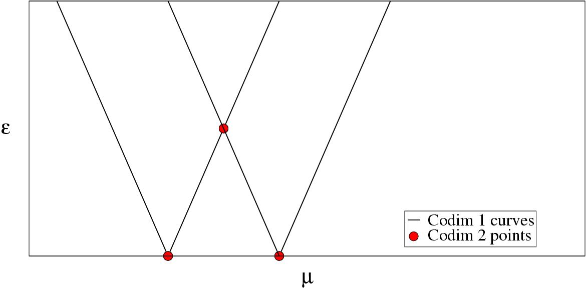
Since we have two parameters in our problem, we are only interested in codimension one and two bifurcations. We first determine the codimension one bifurcation curves and the codimension two bifurcation points for the truncated system in the $\mu$-$\epsilon$ plane, by analyzing the eigenvalues of the linearized operator L. The unstable regions in the $\mu$-$\epsilon$ plane consists of wedges bounded by pairs of codimension one curves that emerge from codimension two points (fig 1).

Figure 1: A Wedge.

We then determine the relevant coefficients for the general normal forms at each of the codimension two points. Using this information, we determine the nature of the bifurcation at the codimension two points and along the pairs of codimension one curves that emanate from these points, at least in the vicinity of these codimension two points.

Lastly, we verify the theoretical predictions by direct numerical simulation of the truncated system, and by comparison with experiments where possible.